EEG data examples#
Here, we demonstrate sbijax using a complicated real world EEG data set. We first load some required libraries and an EEG dataset.
We will take EEG measurements when subjects have their eyes closed or open, respectively, and compute posterior distributions of relevant parameters for each measurement to detect a difference in distributions between the two.
[1]:
import os
import arviz as az
import jax
import numpy as np
import optax
import pandas as pd
import sbijax
import seaborn as sns
%matplotlib inline
import matplotlib.pyplot as plt
import matplotlib.patches as mpatches

from jax import numpy as jnp, random as jr
from tensorflow_probability.substrates.jax import distributions as tfd
[2]:
import mne
import moabb

from jax.scipy.signal import welch
from mne import set_config, get_config
from moabb.datasets import Rodrigues2017
EEG data#
The data set can be readily downloaded using the moabb package and preprocessed using the EEG analysis tool mne.
[3]:
mne_pt = "mne_data"
if not os.path.exists(mne_pt):
    os.mkdir(mne_pt)

set_config('MNE_DATASETS_ALPHAWAVES_PATH', mne_pt)
dataset = Rodrigues2017()
dataset.download()
/var/folders/w8/7mc8k9m916qgh982xqxfgsr00000gn/T/ipykernel_82397/2610150450.py:5: RuntimeWarning: Setting non-standard config type: "MNE_DATASETS_ALPHAWAVES_PATH"
  set_config('MNE_DATASETS_ALPHAWAVES_PATH', mne_pt)
Downloading data from 'https://zenodo.org/record/2348892/files/subject_01.mat' to file '/Users/simon/PROJECTS/2022-bistom/docs/manuscript/sbijax/submission-v1/code/experimental_code/mne_data/MNE-alphawaves-data/record/2348892/files/subject_01.mat/1a7baf6b5525ddbff0c358d0aafba7d2-subject_01.mat'.
SHA256 hash of downloaded file: 4369a2bf7766dc16fdea44ce4d70b96448c2a7784ec097deb0d66b57f29438d3
Use this value as the 'known_hash' argument of 'pooch.retrieve' to ensure that the file hasn't changed if it is downloaded again in the future.
Downloading data from 'https://zenodo.org/record/2348892/files/subject_02.mat' to file '/Users/simon/PROJECTS/2022-bistom/docs/manuscript/sbijax/submission-v1/code/experimental_code/mne_data/MNE-alphawaves-data/record/2348892/files/subject_02.mat/2af6d410a21457fb64c3dd74e9f3951d-subject_02.mat'.
SHA256 hash of downloaded file: f178eac0720679bac17e4cc18b7b958d3fbfe81246f45792699a7e0f9b63da8d
Use this value as the 'known_hash' argument of 'pooch.retrieve' to ensure that the file hasn't changed if it is downloaded again in the future.
Downloading data from 'https://zenodo.org/record/2348892/files/subject_03.mat' to file '/Users/simon/PROJECTS/2022-bistom/docs/manuscript/sbijax/submission-v1/code/experimental_code/mne_data/MNE-alphawaves-data/record/2348892/files/subject_03.mat/9b1a543065884b8a3650078627263591-subject_03.mat'.
SHA256 hash of downloaded file: 9db2e0f7ff016c8ab0fe5a151f085ddb14a20d3fcd91ee0f9c67f736008d925c
Use this value as the 'known_hash' argument of 'pooch.retrieve' to ensure that the file hasn't changed if it is downloaded again in the future.
Downloading data from 'https://zenodo.org/record/2348892/files/subject_04.mat' to file '/Users/simon/PROJECTS/2022-bistom/docs/manuscript/sbijax/submission-v1/code/experimental_code/mne_data/MNE-alphawaves-data/record/2348892/files/subject_04.mat/e88ffc7ee4d9ffc930794f800ed0048c-subject_04.mat'.
SHA256 hash of downloaded file: 987e0f2f621b61815516fa94578252157262cf305b370b0e3d1f771d811bd93d
Use this value as the 'known_hash' argument of 'pooch.retrieve' to ensure that the file hasn't changed if it is downloaded again in the future.
Downloading data from 'https://zenodo.org/record/2348892/files/subject_05.mat' to file '/Users/simon/PROJECTS/2022-bistom/docs/manuscript/sbijax/submission-v1/code/experimental_code/mne_data/MNE-alphawaves-data/record/2348892/files/subject_05.mat/e85d6961d028623625760ae376988d37-subject_05.mat'.
SHA256 hash of downloaded file: 1c0b780192501fab776adf282bd0c39e25c46728aa96c9acb9ce1b0e1deb057b
Use this value as the 'known_hash' argument of 'pooch.retrieve' to ensure that the file hasn't changed if it is downloaded again in the future.
Downloading data from 'https://zenodo.org/record/2348892/files/subject_06.mat' to file '/Users/simon/PROJECTS/2022-bistom/docs/manuscript/sbijax/submission-v1/code/experimental_code/mne_data/MNE-alphawaves-data/record/2348892/files/subject_06.mat/81faad6d15d0e80a91508367a045d32b-subject_06.mat'.
SHA256 hash of downloaded file: 648704b3fbd9ed8398ef329c090453997e4d908f54f9ed725a6513afa81db9fa
Use this value as the 'known_hash' argument of 'pooch.retrieve' to ensure that the file hasn't changed if it is downloaded again in the future.
Downloading data from 'https://zenodo.org/record/2348892/files/subject_08.mat' to file '/Users/simon/PROJECTS/2022-bistom/docs/manuscript/sbijax/submission-v1/code/experimental_code/mne_data/MNE-alphawaves-data/record/2348892/files/subject_08.mat/61822430ce582d208c2cef3eca5bfd1a-subject_08.mat'.
SHA256 hash of downloaded file: ec32952197526c0ad4d25d0eac01a5c47ff76b50cd50a0fd4040ab192ef729e5
Use this value as the 'known_hash' argument of 'pooch.retrieve' to ensure that the file hasn't changed if it is downloaded again in the future.
Downloading data from 'https://zenodo.org/record/2348892/files/subject_09.mat' to file '/Users/simon/PROJECTS/2022-bistom/docs/manuscript/sbijax/submission-v1/code/experimental_code/mne_data/MNE-alphawaves-data/record/2348892/files/subject_09.mat/ea4d45ce573a06145bb10310bf9a089c-subject_09.mat'.
SHA256 hash of downloaded file: c0b529bb3191b3e2d6c8adeab6d1cb486ccb3439e8140153759382d2ffc94fa1
Use this value as the 'known_hash' argument of 'pooch.retrieve' to ensure that the file hasn't changed if it is downloaded again in the future.
Downloading data from 'https://zenodo.org/record/2348892/files/subject_10.mat' to file '/Users/simon/PROJECTS/2022-bistom/docs/manuscript/sbijax/submission-v1/code/experimental_code/mne_data/MNE-alphawaves-data/record/2348892/files/subject_10.mat/2e19861228f7768f33793f133896ec4e-subject_10.mat'.
SHA256 hash of downloaded file: fb0f23e3657bde266bbe376f4fa49430192f41816785fe13845621201ad4a44e
Use this value as the 'known_hash' argument of 'pooch.retrieve' to ensure that the file hasn't changed if it is downloaded again in the future.
Downloading data from 'https://zenodo.org/record/2348892/files/subject_11.mat' to file '/Users/simon/PROJECTS/2022-bistom/docs/manuscript/sbijax/submission-v1/code/experimental_code/mne_data/MNE-alphawaves-data/record/2348892/files/subject_11.mat/86983ff0be3cf29b58eff6e79c7cdeda-subject_11.mat'.
SHA256 hash of downloaded file: 643a4909eeeb77139c2d7af2fa6a87f004afcf792c7d8ef77caac030b5c8c542
Use this value as the 'known_hash' argument of 'pooch.retrieve' to ensure that the file hasn't changed if it is downloaded again in the future.
Downloading data from 'https://zenodo.org/record/2348892/files/subject_12.mat' to file '/Users/simon/PROJECTS/2022-bistom/docs/manuscript/sbijax/submission-v1/code/experimental_code/mne_data/MNE-alphawaves-data/record/2348892/files/subject_12.mat/d1bbf891e77dae4c8e02c44c316edbd3-subject_12.mat'.
SHA256 hash of downloaded file: 216bb0eeed6705cf25b6d751494025fa08d770e90770b98437270614103acd80
Use this value as the 'known_hash' argument of 'pooch.retrieve' to ensure that the file hasn't changed if it is downloaded again in the future.
Downloading data from 'https://zenodo.org/record/2348892/files/subject_13.mat' to file '/Users/simon/PROJECTS/2022-bistom/docs/manuscript/sbijax/submission-v1/code/experimental_code/mne_data/MNE-alphawaves-data/record/2348892/files/subject_13.mat/fbd393840c7767537293a69e8a9a6751-subject_13.mat'.
SHA256 hash of downloaded file: b88df9e5b462d01161040d87a28a59cfb84b500baac3579e431cbd69e4eaa2b7
Use this value as the 'known_hash' argument of 'pooch.retrieve' to ensure that the file hasn't changed if it is downloaded again in the future.
Downloading data from 'https://zenodo.org/record/2348892/files/subject_14.mat' to file '/Users/simon/PROJECTS/2022-bistom/docs/manuscript/sbijax/submission-v1/code/experimental_code/mne_data/MNE-alphawaves-data/record/2348892/files/subject_14.mat/8af67217b5a665aada73906c73d94054-subject_14.mat'.
SHA256 hash of downloaded file: 67ccb112b6a6f2366be543f03a8ec8fc9ee31a1f9104ad1298b31b78b3c9704c
Use this value as the 'known_hash' argument of 'pooch.retrieve' to ensure that the file hasn't changed if it is downloaded again in the future.
Downloading data from 'https://zenodo.org/record/2348892/files/subject_15.mat' to file '/Users/simon/PROJECTS/2022-bistom/docs/manuscript/sbijax/submission-v1/code/experimental_code/mne_data/MNE-alphawaves-data/record/2348892/files/subject_15.mat/9258e7a0bb6786c82088c9235e13715b-subject_15.mat'.
SHA256 hash of downloaded file: 7efb82cee33bace27f9442ce22dc69022c8dfd0759b3d6cb4785bcb6fb21e48e
Use this value as the 'known_hash' argument of 'pooch.retrieve' to ensure that the file hasn't changed if it is downloaded again in the future.
Downloading data from 'https://zenodo.org/record/2348892/files/subject_16.mat' to file '/Users/simon/PROJECTS/2022-bistom/docs/manuscript/sbijax/submission-v1/code/experimental_code/mne_data/MNE-alphawaves-data/record/2348892/files/subject_16.mat/c96d9e1f5d8c94c2ea387ea6a9dcc8b9-subject_16.mat'.
SHA256 hash of downloaded file: 5cac69336049d9e445eaeab17d36d08c6d2d6c7e8006ee257c05e45592610586
Use this value as the 'known_hash' argument of 'pooch.retrieve' to ensure that the file hasn't changed if it is downloaded again in the future.
Downloading data from 'https://zenodo.org/record/2348892/files/subject_17.mat' to file '/Users/simon/PROJECTS/2022-bistom/docs/manuscript/sbijax/submission-v1/code/experimental_code/mne_data/MNE-alphawaves-data/record/2348892/files/subject_17.mat/0413a86bdc5eeaf38df7a1d281f650be-subject_17.mat'.
SHA256 hash of downloaded file: aa94ead9a6d16c6ac6455ad6c4bec29ac95a7ec621e9182257241c5ba3fdca34
Use this value as the 'known_hash' argument of 'pooch.retrieve' to ensure that the file hasn't changed if it is downloaded again in the future.
Downloading data from 'https://zenodo.org/record/2348892/files/subject_18.mat' to file '/Users/simon/PROJECTS/2022-bistom/docs/manuscript/sbijax/submission-v1/code/experimental_code/mne_data/MNE-alphawaves-data/record/2348892/files/subject_18.mat/a445cd7406c8a07ded4144094cd411c9-subject_18.mat'.
SHA256 hash of downloaded file: fdb133eb968c95b3e46eb618b053d0a559e6638b4c739d1e3d7cf20a2ad49093
Use this value as the 'known_hash' argument of 'pooch.retrieve' to ensure that the file hasn't changed if it is downloaded again in the future.
Downloading data from 'https://zenodo.org/record/2348892/files/subject_19.mat' to file '/Users/simon/PROJECTS/2022-bistom/docs/manuscript/sbijax/submission-v1/code/experimental_code/mne_data/MNE-alphawaves-data/record/2348892/files/subject_19.mat/0a90a1e6d5f138adb19b979954d6bd33-subject_19.mat'.
SHA256 hash of downloaded file: e2ce803fa962e941ce0ff80dbd40c38e86be36c9ec7a5ec1f6fcc2560690adec
Use this value as the 'known_hash' argument of 'pooch.retrieve' to ensure that the file hasn't changed if it is downloaded again in the future.
Downloading data from 'https://zenodo.org/record/2348892/files/subject_20.mat' to file '/Users/simon/PROJECTS/2022-bistom/docs/manuscript/sbijax/submission-v1/code/experimental_code/mne_data/MNE-alphawaves-data/record/2348892/files/subject_20.mat/6a81ea79d0317c0946aad87f9491273e-subject_20.mat'.
SHA256 hash of downloaded file: 301c43250c8649957913a8001340e4b10299e33add25cb6a5a11aa1bf0ea2df8
Use this value as the 'known_hash' argument of 'pooch.retrieve' to ensure that the file hasn't changed if it is downloaded again in the future.
Following previous work (the our manuscript for more information), we filter the data at 3Hz and 40Hz and resample them.
[4]:
raw = dataset._get_single_subject_data(subject=2)['0']['0']
raw = raw.filter(l_freq=3, h_freq=40, verbose=False)
raw = raw.resample(sfreq=128, verbose=False)
We then extract the EEG recordings from the Oz channel and visualize the data.
[5]:
events = mne.find_events(raw=raw, shortest_event=1, verbose=False)
event_id = {'closed': 1, 'open': 2}
epochs = mne.Epochs(raw, events, event_id, tmin=0.0, tmax=8.0, baseline=None, verbose=False)
epochs = epochs.load_data().pick_channels(['Oz'])
Using data from preloaded Raw for 10 events and 1025 original time points ...
0 bad epochs dropped
NOTE: pick_channels() is a legacy function. New code should use inst.pick(...).
[6]:
X_closed = epochs['closed'].get_data().squeeze()
f, S_closed = welch(X_closed, fs=epochs.info['sfreq'], nperseg=64, axis=1)
S_closed_db = 10 * np.log10(S_closed)

X_opened = epochs['open'].get_data().squeeze()
f, S_opened = welch(X_opened, fs=epochs.info['sfreq'], nperseg=64, axis=1)
S_opened_db = 10 * np.log10(S_opened)
[7]:
color_closed = "#700e01"
color_open = "#c79999"
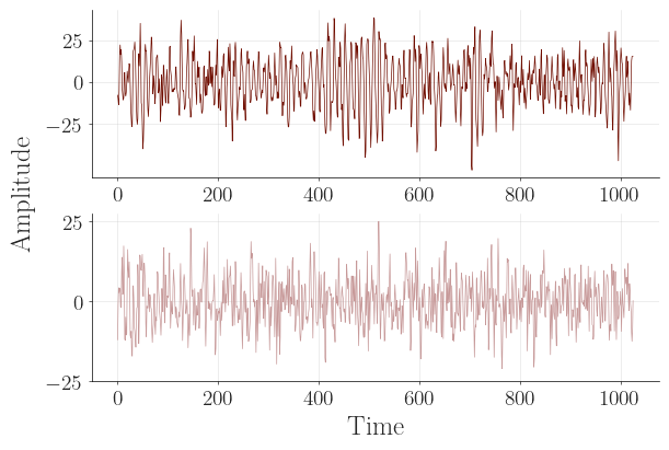
To compute posterior distributions later, we randomly select one sample from the closed-eyes EEGs and one from the open-eyes EEGs.
[8]:
with plt.style.context("sbijax"):
fig, laxes = plt.subplots(layout="constrained", figsize=(6, 4), nrows=2)
laxes[0].plot(X_closed[2, :], color=color_closed, label="closed", linewidth=.5)
laxes[1].plot(X_opened[2, :], color=color_open, label="opened", linewidth=.5)
laxes[0].yaxis.set_ticks([-25, 0, 25])
laxes[1].yaxis.set_ticks([-25, 0, 25])
laxes[0].tick_params(axis='both',labelsize=14)
laxes[1].tick_params(axis='both',labelsize=14)
laxes[0].grid(linewidth=0.5)
laxes[1].grid(linewidth=0.5)
laxes[0].spines['bottom'].set_color('black')
laxes[1].spines['bottom'].set_color('black')
laxes[0].spines['left'].set_color('black')
laxes[1].spines['left'].set_color('black')
laxes[1].set_xlabel("Time", fontsize=18)
laxes[0].set_ylabel("Amplitude", fontsize=18)
laxes[0].yaxis.set_label_coords(-0.1, -0.1)
plt.show()
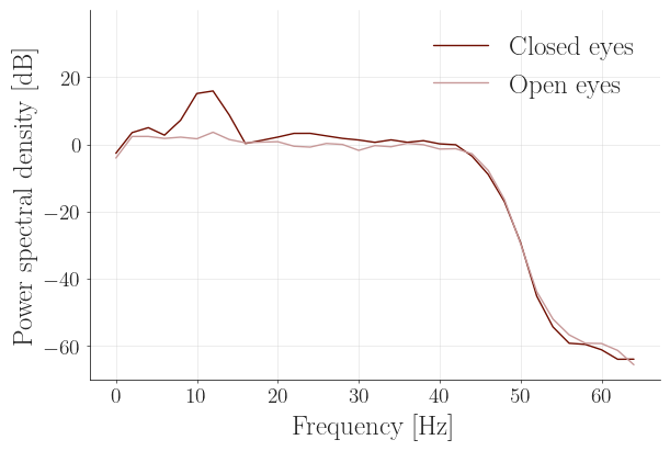
with plt.style.context("sbijax"):
fig, raxes = plt.subplots(layout="constrained", figsize=(6, 4))
raxes.plot(f, S_closed_db[2], color=color_closed, lw=1, label="Closed eyes")
raxes.plot(f, S_opened_db[2], color=color_open, lw=1, label="Open eyes")
raxes.yaxis.set_ticks([-60, -40, -20, 0, 20], )
raxes.set_ylim(-70, 40)
raxes.spines['bottom'].set_color('black')
raxes.spines['left'].set_color('black')
raxes.tick_params(axis='both',labelsize=14)
raxes.set_xlabel("Frequency [Hz]", fontsize=18)
raxes.set_ylabel("Power spectral density [dB]", fontsize=18)
raxes.legend(frameon=False, fontsize=18)
raxes.grid(linewidth=0.5)
plt.show()
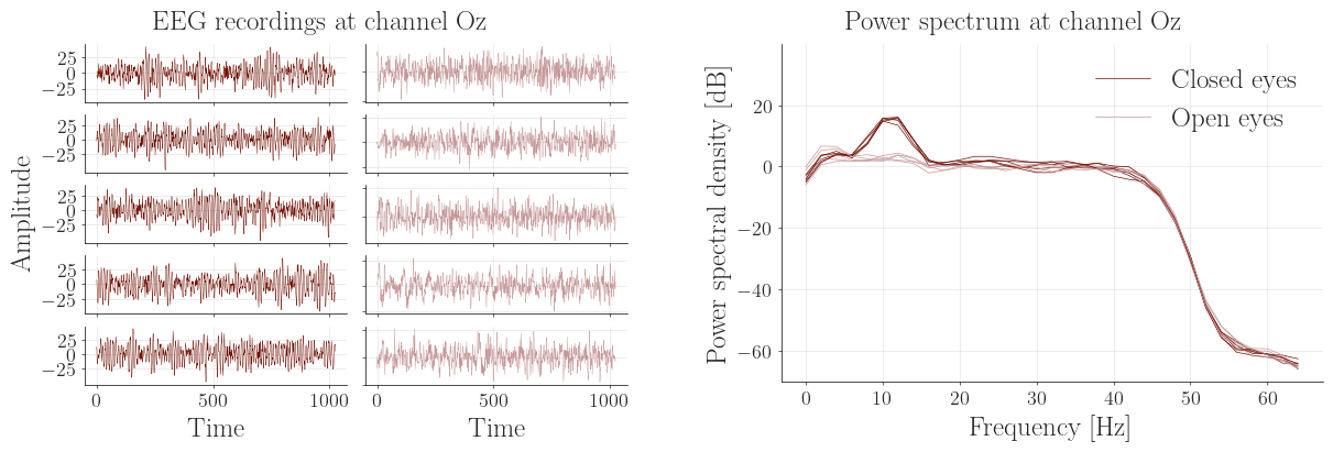
For completeness, we plot the entire data set, too.
[9]:
fig = plt.figure(layout="constrained", figsize=(12, 4))
subfigs = fig.subfigures(1, 2, wspace=0.1, width_ratios=[1.5, 1.5])
with plt.style.context("sbijax"):
    subfigs[0].suptitle("EEG recordings at channel Oz", fontsize=18)
    subfigs[1].suptitle("Power spectrum at channel Oz", fontsize=18)
    laxes = subfigs[0].subplots(5, 2)
    for i in range(5):
        laxes[i, 0].plot(X_closed[i, :], color=color_closed, label="closed", linewidth=.31)
        laxes[i, 1].plot(X_opened[i, :], color=color_open, label="opened", linewidth=.31)
        if i != 4:
            laxes[i, 0].xaxis.set_ticklabels([])
            laxes[i, 1].xaxis.set_ticklabels([])
        laxes[i, 0].yaxis.set_ticks([-25, 0, 25])
        laxes[i, 1].yaxis.set_ticklabels([])
        laxes[i, 0].grid(linewidth=0.5)
        laxes[i, 1].grid(linewidth=0.5)
        laxes[i, 0].spines['bottom'].set_color('black')
        laxes[i, 0].spines['left'].set_color('black')
        laxes[i, 1].spines['bottom'].set_color('black')
        laxes[i, 1].spines['left'].set_color('black')
        laxes[i, 0].tick_params(axis='both',labelsize=13)
        laxes[i, 1].tick_params(axis='both',labelsize=13)
    laxes[2, 0].set_ylabel("Amplitude", fontsize=18)
    laxes[4, 0].set_xlabel("Time", fontsize=18)
    laxes[4, 1].set_xlabel("Time", fontsize=18)

    raxes = subfigs[1].subplots(1, 1)
    for i in range(5):
        if i ==0:
            raxes.plot(f, S_closed_db[i], color=color_closed, lw=.5, label="Closed eyes")
            raxes.plot(f, S_opened_db[i], color=color_open, lw=.5, label="Open eyes")
        else:
            raxes.plot(f, S_closed_db[i], color=color_closed, lw=.5)
            raxes.plot(f, S_opened_db[i], color=color_open, lw=.5)
    raxes.yaxis.set_ticks([-60, -40, -20, 0, 20])
    raxes.set_ylim(-70, 40)
    raxes.spines['bottom'].set_color('black')
    raxes.spines['left'].set_color('black')
    raxes.set_ylabel("Power spectral density [dB]", fontsize=18)
    raxes.set_xlabel("Frequency [Hz]", fontsize=18)
    raxes.legend(frameon=False, fontsize=18)
    raxes.grid(linewidth=0.5)
    raxes.tick_params(axis='both',labelsize=13)
plt.show()
Prior and simulator#
We next set up the prior and simulator. For the simulator, we use the sdbmpABC package which neatly implements the Jansen-Rit SDE (unfortunately it is written in R/C++).
[10]:
def prior_fn():
    prior = tfd.JointDistributionNamed(dict(
        C=tfd.Uniform(10.0, 250.0),
        mu=tfd.Uniform(50.0, 500.0),
        sigma=tfd.Uniform(100, 5000),
        gain=tfd.Uniform(-20, 20),
    ), batch_ndims=0)
    return prior

prior = prior_fn()
[11]:
from jrnmm import simulate
[12]:
def jansen_rit_fn(len_timeseries=1025, t_end=8.0):
    from jrnmm import simulate as simulate_jrnmm

    burnin = 0.0
    h = 1 / 128 # sampling rate is 1/F where F=128
    def fn(seed, theta):
        yt = simulate_jrnmm(
            seed,
            dt=h,
            t_end=t_end + burnin + h,
            initial_states=jnp.array([0.08, 18, 15, -0.5, 0.0, 0.0]),
            Cs=theta['C'],
            mus=theta['mu'],
            sigmas=theta['sigma'],
            gains=theta['gain'],
        )
        yt = yt[:, int(burnin/h):, 0]
        yt = yt - jnp.mean(yt, axis=1, keepdims=True)
        return yt

    return fn

simulate_jansen_rit = jansen_rit_fn(len_timeseries=1025, t_end=8.0)
We then construct a simulator suitable for sbijax.
[13]:
def simulator(seed, theta, len_timeseries=1025, t_end=8.0, batch_size=1_000):
    n = theta['C'].shape[0]
    seeds = jr.split(seed, n)

    ys = []
    n_batches = n // batch_size + int(np.ceil(n % batch_size / batch_size))
    for i in range(n_batches):
        sl = slice(i * batch_size, (i + 1) * batch_size)
        theta_sub = jax.tree.map(lambda x: x[sl], theta)
        y = simulate_jansen_rit(seed, theta_sub)
        ys.append(y.astype(jnp.float32))
    ys = jnp.vstack(ys)
    return ys
In a final step before inferring the posteriors, we simulate \(100\ 000\) synthetic trajectories. We save them, a reference trjectory for testing, and the real data as a pickle file in order to avoid lengthy computations.
[14]:
def get_experimental_data(prior, n_simulations=100_000):
    # synthetic data example
    theta_synthetic = dict(zip(['C', 'mu', 'sigma', 'gain'], [135, 220, 2000, 0]))
    y_synthetic = simulate_jansen_rit(jr.PRNGKey(1), theta_synthetic)

    # experimental data
    y_experimental_closed = X_closed[[4]]
    y_experimental_opened = X_opened[[4]]

    # simulations
    theta_train = prior.sample(seed=jr.PRNGKey(0), sample_shape=(n_simulations,))
    y_train = simulator(jr.PRNGKey(1), theta_train)

    di = dict(
        theta_synthetic=theta_synthetic,
        y_synthetic=y_synthetic,
        y_experimental_closed=y_experimental_closed,
        y_experimental_opened=y_experimental_opened,
        theta_train=theta_train,
        y_train=y_train
    )
    jax.config.update("jax_enable_x64", False)
    return di

eeg_data = get_experimental_data(prior)
Summary statistics#
As described in the manuscript, we do inference on a collection of summary statistics for which we take the spectral density evaluated at several bins instead of the entire time series.
[15]:
def summarize(y, n_summaries=33, fs=epochs.info['sfreq']):
    _, summaries = welch(y, fs=fs, nperseg=2 * (n_summaries - 1), axis=1)
    return summaries
[16]:
summaries_train = summarize(eeg_data["y_train"])
Neural posterior estimation#
We now do posterior inference. We choose to use neural posterior estimation here, but any other method implemented in sbijax would also work. Neural posterior, however, has the advantage that we only have to model a four-dimensional space (i.e., the dimensionality of the posterior) and not the data space, which makes it efficient in this scenario.
We train in an amortized fashion such that we can compute posteriors for multiple observations (i.e., closed vs opened eyes).
Notice that we do not provide the simulator function here. Since we train in an amortized fashion and already have a set of simulated samples, the simulator is not needed here. In many inferential problems in the natural sciences it is common that new data cannot be simulated, but a batch of previously simulated samples is available. sbijax supports this scenario like this as shown below.
[17]:
from sbijax import NPE
from sbijax.nn import make_maf
[18]:
n_dim_data = 33 # number of summary statistics from prior literature
n_dim_theta = 4 # posterior dimensionality
n_layers, hidden_sizes = 10, (64, 64)
neural_network = make_maf(n_dim_theta, n_layers, hidden_sizes=hidden_sizes)

fns = prior_fn, None
[19]:
summaries_train.shape
[19]:
(100000, 33)
[20]:
data = {"y": summaries_train, "theta": eeg_data["theta_train"]}
estim = NPE(fns, neural_network, use_event_space_bijections=False)
params, info = estim.fit(
    jr.PRNGKey(1),
    data=data,
    optimizer=optax.adam(0.0001),
    n_early_stopping_delta=0.01,
    n_early_stopping_patience=10,
)
20%|███████████████████████████▉ | 198/1000 [05:35<22:39, 1.70s/it]
Synthetic data example#
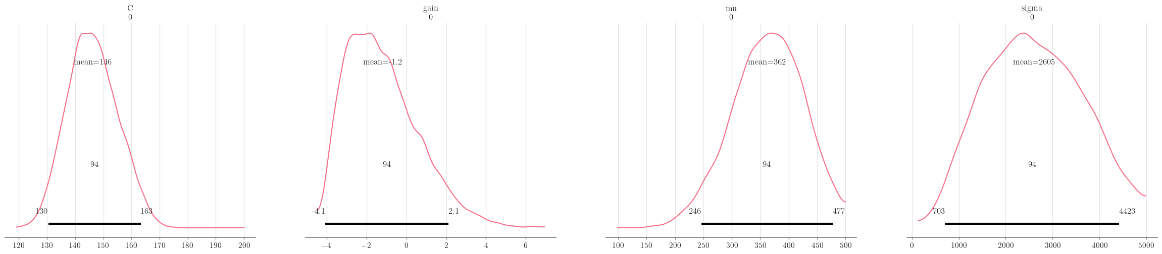
We evaluate first if we are able to approximately infer the true parameter values for a synthetic samples.
[21]:
posterior_synthetic, _ = estim.sample_posterior(
    jr.PRNGKey(2),
    params,
    observable=summarize(eeg_data["y_synthetic"].reshape(1, -1)),
    n_samples=10_000,
)
[22]:
eeg_data["theta_synthetic"]
[22]:
{'C': 135, 'mu': 220, 'sigma': 2000, 'gain': 0}
[23]:
az.plot_posterior(posterior_synthetic)
plt.show()
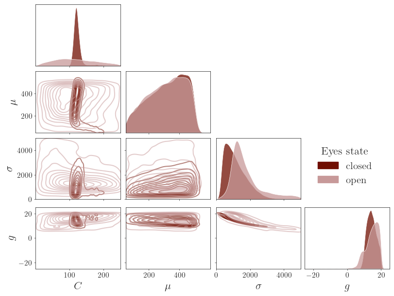
Inference of posterior distributions for closed and opened eyes EEG data#
We, finally, infer the posterior distributions of EEG data when eyes where closed or openened, respectively. Having an amortized posterior model, we can just plug in different observations and sample from the trained normalizing flow model. For the open eyes state, this might take considerably longer since the data cannot be well described by the simulator model.
[24]:
posterior_closed, _ = estim.sample_posterior(
    jr.PRNGKey(2),
    params,
    observable=summarize(eeg_data["y_experimental_closed"]),
    n_samples=10_000
)
[25]:
posterior_open, _ = estim.sample_posterior(
    jr.PRNGKey(2),
    params,
    observable=summarize(eeg_data["y_experimental_opened"]),
    n_samples=10_000,
)
We convert the inference data to flat dictionaries for ease of plotting, and then visualize the posterior distributions of both eye states.
[26]:
posterior_open = sbijax.inference_data_as_dictionary(posterior_open.posterior)
posterior_closed = sbijax.inference_data_as_dictionary(posterior_closed.posterior)
[27]:
symbols = ["$C$", "$\\mu$", "$\\sigma$", "$g$"]
keys = ['C', 'mu', 'sigma', 'gain']
[28]:
lims = {
    "C": ((0, 250), (100, 200)),
    "mu": ((50.0, 600.0), (200, 400)),
    "sigma": ((0, 5000), (0, 2000, 4000)),
    "gain": ((-25, 25), (-20, 0, 20))
}
[29]:
with plt.style.context("sbijax"):
    _, axes = plt.subplots(figsize=(8, 6), nrows=4, ncols=4, layout="constrained")
    for i, key_i in enumerate(keys):
        for j, key_j in enumerate(keys):
            ax = axes[i, j]
            ax.grid(False)
            ax.spines['bottom'].set_color('black')
            ax.spines['left'].set_color('black')
            ax.spines['right'].set_visible(True)
            ax.spines['right'].set_color('black')
            ax.spines['top'].set_visible(True)
            ax.spines['top'].set_color('black')
            ax.set_ylabel(None)
            ax.set_xlabel(None)
            if i < j:
                ax.axis('off')
            elif i != j:
                ddf = pd.DataFrame({key_j: np.squeeze(posterior_closed[key_j]), key_i: np.squeeze(posterior_closed[key_i])})
                sns.kdeplot(data=ddf, x=key_j, y=key_i, ax=ax, color=color_closed, alpha=.5)
                ddf = pd.DataFrame({key_j: np.squeeze(posterior_open[key_j]), key_i: np.squeeze(posterior_open[key_i])})
                sns.kdeplot(data=ddf, x=key_j, y=key_i, ax=ax, color=color_open, alpha=.5)
                ax.set_ylim(*lims[key_i][0])
                ax.set_xlim(*lims[key_j][0])
                ax.set_yticks(lims[key_i][1])
                ax.set_xticks(lims[key_j][1])
                ax.set_xlabel(None)
                ax.set_ylabel(None)

                if j == 0:
                    ax.set_ylabel(symbols[i], fontsize=16)
                else:
                    ax.set_yticklabels([])
                if i == 3:
                    ax.set_xlabel(symbols[j], fontsize=16)
                else:
                    ax.set_xticklabels([])
            else:
                ddf = pd.DataFrame({key_j: np.squeeze(posterior_closed[key_j])})
                sns.kdeplot(data=ddf, x=key_j, ax=ax, color=color_closed, multiple="stack", linewidth=.5, edgecolor="white", label="Closed eyes")
                ddf = pd.DataFrame({key_j: np.squeeze(posterior_open[key_j])})
                sns.kdeplot(data=ddf, x=key_j, ax=ax, color=color_open, multiple="stack", linewidth=.5, edgecolor="white",label="Open eyes")
                ax.set_xlabel(None)
                ax.set_ylabel(None)
                if i != 3:
                    ax.set_xticklabels([])
                ax.set_yticks([])
                ax.set_yticklabels([])
                if i == 3:
                    ax.set_xlabel(symbols[i], fontsize=16)
                ax.set_xlim(*lims[key_i][0])
                ax.set_xticks(lims[key_i][1])
axes[2, 3].legend(
    title="Eyes state",
    handles=[
        mpatches.Patch(color=color_closed, label='closed'),
        mpatches.Patch(color=color_open, label='open'),
    ],
    frameon=False,
    bbox_to_anchor=(0.9, 1),
    fontsize=15,
    title_fontsize=16
)
plt.show()
Session info#
[30]:
import session_info

session_info.show(html=False)
-----
arviz                       0.19.0
haiku                       0.0.12
jax                         0.4.31
jaxlib                      0.4.31
jrnmm                       0.1.0.post1
matplotlib                  3.9.2
mne                         1.8.0
moabb                       1.1.1
numpy                       1.26.4
optax                       0.2.4
pandas                      1.5.3
sbijax                      0.3.3
seaborn                     0.12.2
session_info                1.0.0
tensorflow_probability      0.25.0
-----
IPython             8.31.0
jupyter_client      8.6.3
jupyter_core        5.7.2
jupyterlab          4.3.1
-----
Python 3.11.7 (main, Dec  9 2023, 06:06:18) [Clang 14.0.3 (clang-1403.0.22.14.1)]
macOS-13.0.1-arm64-arm-64bit
-----
Session information updated at 2025-01-04 20:56