A more detailed introduction

The following notebook expands a bit on the “Getting started” one.

import jax
import sbijax
%matplotlib inline
import matplotlib.pyplot as plt

import matplotlib.pyplot as plt

def plot_posterior_hist(samples, key="theta", bins=40):
    theta = samples[key].reshape(-1, samples[key].shape[-1])
    d = theta.shape[-1]
    fig, axes = plt.subplots(1, d, figsize=(3 * d, 3))
    axes = [axes] if d == 1 else list(axes)
    for i, ax in enumerate(axes):
        ax.hist(theta[:, i], bins=bins, color="#700e01")
        ax.set_title(f"{key}[{i}]")
    fig.tight_layout(); return fig

Model definition

To do approximate inference using sbijax, a user first has to define a prior model and a simulator function which can be used to generate synthetic data. We will be using a simple bivariate Gaussian as an example with the following generative model:

\begin{align} \mu &\sim \mathcal{N}_2(0, I)\\ \sigma &\sim \mathcal{N}^+(1)\\ y & \sim \mathcal{N}_2(\mu, \sigma^2 I) \end{align}

Using TensorFlow Probability, the prior model and simulator are implemented like this:

from jax import numpy as jnp, random as jr
from tensorflow_probability.substrates.jax import distributions as tfd

def prior_fn():
    prior = tfd.JointDistributionNamed(dict(
        mean=tfd.Normal(jnp.zeros(2), 1.0),
        scale=tfd.HalfNormal(jnp.ones(1)),
    ), batch_ndims=0)
    return prior

def simulator_fn(seed: jr.PRNGKey, theta: dict[str, jax.Array]):
    p = tfd.Normal(jnp.zeros_like(theta["mean"]), 1.0)
    y = theta["mean"] + theta["scale"] * p.sample(seed=seed)
    return y

prior = prior_fn()
theta = prior.sample(seed=jr.PRNGKey(0), sample_shape=())
theta

{'scale': Array([0.47995827], dtype=float32),
 'mean': Array([0.62157685, 0.8429717 ], dtype=float32)}

prior.log_prob(theta)

Array(-2.7273278, dtype=float32)

simulator_fn(seed=jr.PRNGKey(1), theta=theta)

Array([0.54745346, 0.88362765], dtype=float32)

theta = prior.sample(seed=jr.PRNGKey(2), sample_shape=(2,))
theta

{'scale': Array([[0.48404777],
        [0.3731677 ]], dtype=float32),
 'mean': Array([[ 1.2550716 ,  0.27969918],
        [-0.66132253, -0.79632473]], dtype=float32)}

prior.log_prob(theta)

Array([-3.0075376, -2.6690357], dtype=float32)

simulator_fn(seed=jr.PRNGKey(3), theta=theta)

Array([[ 0.5550142 ,  1.0248331 ],
       [-0.51858354, -0.0609225 ]], dtype=float32)

Algorithm definition

Having defined a model of interest, i.e., the prior and simulator functions, we construct an inferential method. We can use a pre-implemented method to construct a normalizing flow, but for the sake of demonstration we implement a MAF from scratch.

import haiku as hk
import surjectors
import surjectors.nn
import surjectors.util
from sbijax import nle

n_dim_data = 2
n_layers, hidden_sizes = 5, (64, 64)

def make_custom_affine_maf(n_dimension, n_layers, hidden_sizes):
    def _bijector_fn(params):
        means, log_scales = surjectors.util.unstack(params, -1)
        return surjectors.ScalarAffine(means, jnp.exp(log_scales))

    def _flow(method, **kwargs):
        layers = []
        order = jnp.arange(n_dimension)
        for _ in range(5):
            layer = surjectors.MaskedAutoregressive(
                bijector_fn=_bijector_fn,
                conditioner=surjectors.nn.MADE(
                    n_dimension,
                    list(hidden_sizes),
                    2,
                    w_init=hk.initializers.TruncatedNormal(0.001),
                    b_init=jnp.zeros,
                ),
            )
            order = order[::-1]
            layers.append(layer)
            layers.append(surjectors.Permutation(order, 1))
        chain = surjectors.Chain(layers[:-1])
        base_distribution = tfd.Independent(
            tfd.Normal(jnp.zeros(n_dimension), jnp.ones(n_dimension)),
            1,
        )
        td = surjectors.TransformedDistribution(base_distribution, chain)
        return td(method, **kwargs)

    td = hk.transform(_flow)
    return td

neural_network = make_custom_affine_maf(n_dim_data, n_layers, hidden_sizes)
model = nle(prior, neural_network)

Training and Inference

Inference is then as easy as simulating some data, fitting the data to the model, a sampling from the approximate posterior. The data set is a dictionary of dictionaries (a PyTree in JAX lingo). It contains samples for the simulator function, called y, and parameter samples from the prior model, called theta.

from sbijax import simulate

data = simulate(
    jr.PRNGKey(1),
    prior,
    simulator_fn,
    n=10_000,
)
data

{'y': Array([[ 0.07692909,  0.7882271 ],
        [-1.2418504 , -0.25333643],
        [ 1.1943562 , -2.124853  ],
        ...,
        [ 1.3316323 ,  0.5488601 ],
        [ 4.862982  , -4.1227694 ],
        [-0.00955033,  0.989019  ]], dtype=float32),
 'theta': {'scale': Array([[0.9232396 ],
         [0.36471593],
         [0.6795394 ],
         ...,
         [0.11454558],
         [1.260745  ],
         [0.5012804 ]], dtype=float32),
  'mean': Array([[ 0.30212572,  0.67478853],
         [-0.963459  ,  0.086253  ],
         [ 0.39044896, -2.2378268 ],
         ...,
         [ 1.3652769 ,  0.6302657 ],
         [ 2.7543025 , -1.9100804 ],
         [-0.16545922,  0.6475435 ]], dtype=float32)}}

We then fit the model using the typical flow matching loss.

params, info = model.fit(
    jr.PRNGKey(2),
    data
)

 27%|██████████████████████████████                                                                                | 273/1000 [03:19<08:52,  1.37it/s]

Finally, we sample from the posterior distribution for a specific observation \(y_{\text{obs}}\).

y_obs = jnp.array([-1.0, 1.0])
samples, _ = model.sample(
    jr.PRNGKey(3), params, y_obs, n_chains=4, n_samples=10_000, n_warmup=5_000
)

Model diagnostics and visualization

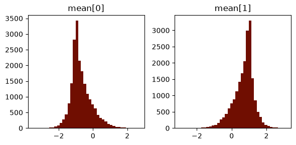
Sbijax provides basic functionality to analyse posterior draws. We show some visualizations below.

plot_posterior_hist(samples, "mean")
plt.show()

plt.plot(info.losses[1:])
plt.xlabel("step")
plt.ylabel("loss")
plt.show()

print("ESS:", sbijax.ess(samples))
print("R-hat:", sbijax.rhat(samples))

ESS: {'mean': Array([20649.303, 18767.834], dtype=float32), 'scale': Array(20291.781, dtype=float32)}
R-hat: {'mean': Array([1.0000986, 1.0001243], dtype=float32), 'scale': Array(1.0015361, dtype=float32)}

Sequential inference

sbijax supports sequential (multi-round) training through the standalone run_sequential driver. It simulates from the current posterior each round, appends to the dataset, and refits, so the estimator itself stays single-round and stateless.

from sbijax import run_sequential

params, info = run_sequential(
    jr.PRNGKey(1),
    model,
    prior,
    simulator_fn,
    y_obs,
    n_rounds=2,
    n_simulations_per_round=2_000,
)

_ , _ = model.sample(jr.PRNGKey(3), params, y_obs)

 29%|████████████████████████████████▎                                                                             | 294/1000 [01:51<04:28,  2.63it/s]
  2%|█▊                                                                                                             | 16/1000 [00:08<08:55,  1.84it/s]

Session info

import session_info

session_info.show(html=False)